This vignette illustrates how to use harvesting scenarii with matreex package. An harvesting scenario provides the rules and the periodicity to trigger harvesting of trees in each size classes. The harvested trees are saved and exported for each simulation time step.
The basic matreex functions are shown in a previous introduction vignette.
Simulations input
Define a species
The first step is the IPM integration. This part is common with basic usage of the package, so nothing is very important here.
Please keep in mind this computation is intensive and may take few minutes !
library(matreex)
library(dplyr)
#>
#> Attaching package: 'dplyr'
#> The following objects are masked from 'package:stats':
#>
#>     filter, lag
#> The following objects are masked from 'package:base':
#>
#>     intersect, setdiff, setequal, union
library(ggplot2)

# Load fitted model for a species
# fit_species # list of all species in dataset
data("fit_Picea_abies")

# Load associated climate
data("climate_species")
climate <- subset(climate_species, N == 2 & sp == "Picea_abies", select = -sp)
# see ?climate_species to understand the filtering of N.
climate
#>        sgdd       wai        sgddb      waib      wai2   sgdd2      PC1
#> 62 1444.667 0.4519387 0.0006922012 0.6887343 0.2042486 2087062 1.671498
#>           PC2 N       SDM
#> 62 0.02602064 2 0.6760556

Picea_ipm <- make_IPM(
    species = "Picea_abies",
    climate = climate,
    fit = fit_Picea_abies,
    clim_lab = "optimum clim",
    mesh = c(m = 700, L = 90, U = get_maxdbh(fit_Picea_abies) * 1.1),
    BA = 0:80, # Default values are 0:200, smaller values speed up this vignette.
    verbose = TRUE
)
#> Launching integration loop
#> GL integration occur on 32 cells
#> midbin integration occur on 25 cells
#> Loop done.
#> Time difference of 54.3 secs
Harvesting scenario are defined at different levels: at the species level with the species harvesting function and its associated parameters, at the forest level with a set of parameters, and at the simulation level with the target of the harvesting scenario. Depending on the scenario used, not all the parameters are used. The table below summarise the required parameters for each scenario. Each scenario have an example in the following document.
| Harvesting scenario | Species harvesting function | Species parameters | Forest parameters | Simulation parameters |
|---|---|---|---|---|
| default |
def_harv() or custom by user. |
\(\emptyset\) | harv_rules["freq"] |
\(\emptyset\) |
| Uneven | Uneven_harv() |
harv_lim |
harv_rules |
targetBA |
| Even | Even_harv() |
rdi_coef |
harv_rules |
targetRDI targetKg final_harv
|
Short example : When using an Uneven scenario, each species needs to
use the Uneven_harv() function with harv_lim
parameters. The forest will need to have harv_rules
parameters. The sim_deter_forest() require
targetBA argument. If targetRDI is defined, it
will not be used.
Default scenario
Presentation
The default scenario is based on Kunstler et al. (2021). This mean there is a constant harvest rate triggered each year. This harvest rate is uniform over the size distribution. This is the scenario used by default.
This rate is coded in def_harv() function as shown below
and the frequency (each year) is given in
harv_rules["freq"]. Note that the harvesting is applied to
all size class except the age-classes used in delay (with
* (ct > 0)).
def_harv
#> function (x, species, ...)
#> {
#>     dots <- list(...)
#>     ct <- dots$ct
#>     rate <- 0.006 * (ct > 0)
#>     return(x * rate)
#> }
#> <bytecode: 0x55b68c1bc728>
#> <environment: namespace:matreex>
Picea_sp <- species(IPM = Picea_ipm, init_pop = def_initBA(30))
Picea_for <- forest(species = list(Picea = Picea_sp),
                    harv_rules = c(freq = 1))
With this scenario, the simulation can be launched without any additional parameter.
set.seed(42) # The seed is here to replicate the random population initialisation.
Picea_sim <- sim_deter_forest(
    Picea_for,
    tlim = 200, equil_time = 200, equil_dist = 10, equil_diff = 1,
    harvest = "default", # this is the default value but we write it.
    SurfEch = 0.03,
    verbose = TRUE
)
#> Starting while loop. Maximum t = 200
#> Simulation ended after time 200
#> BA stabilized at 44.68 with diff of 1.12 at time 200
#> Time difference of 1.11 secs
Once the simulation is done, we can extract the basal area and the number of individual at each step of the simulation, but also a new variable \(H\). This is the sum of densities of harvested trees of all size classes at each time step. The density of harvested trees is also exported for each size mesh \(h_i\).
In this case, \(H\) is correlated with \(N\) since it’s a constant percentage not linked with a size distribution. The first step being the initialization step, it’s normal to have no harvest.
Picea_sim  %>%
    dplyr::filter(var %in% c("BAsp", "N", "H"), ! equil) %>%
    ggplot(aes(x = time, y = value)) +
    facet_wrap(~ var, scales = "free_y") +
geom_line(linewidth = .2) + geom_point(size = 0.4) 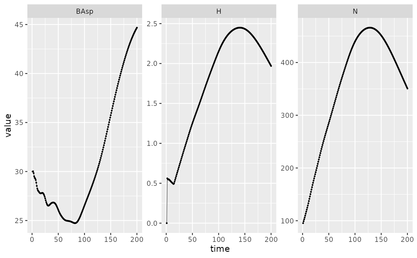
Modulation
This section will just illustrate variation of the default scenario. First we modify the frequency of the harvest. When the harvest is not triggered, the value returned is 0.
set.seed(42) # The seed is here for initial population random functions.
Picea_sim_f20 <- sim_deter_forest(
    forest(species = list(Picea = Picea_sp),
                      harv_rules = c(freq = 20)),
    tlim = 50, equil_time = 50, equil_dist = 10, equil_diff = 1,
    harvest = "default",
    SurfEch = 0.03,
    verbose = TRUE
)
#> Starting while loop. Maximum t = 50
#> Simulation ended after time 50
#> BA stabilized at 32.94 with diff of 0.81 at time 50
#> Time difference of 0.265 secs
Picea_sim_f20  %>%
    dplyr::filter(var %in% c("BAsp", "N", "H"), ! equil) %>%
    ggplot(aes(x = time, y = value)) +
    facet_wrap(~ var, scales = "free_y") +
geom_line(linewidth = .2) + geom_point(size = 0.4) 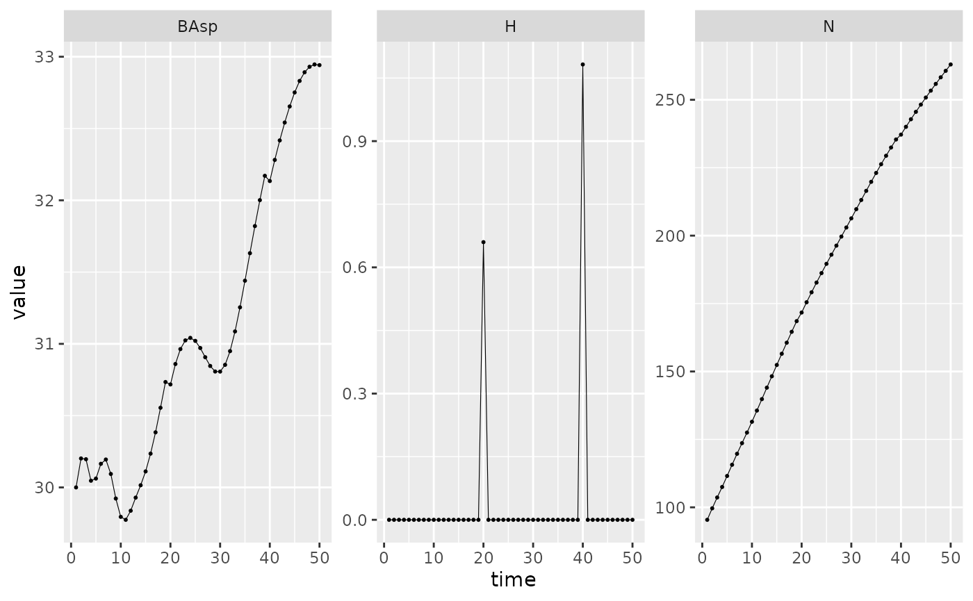
A more advanced modification of the harvest function is ilustratted below. Obviously, this type of modification have not been thoroughly tested and thus is more prone to error so don’t hesitate to contact matreex maintainer in case of trouble. For example, we add a function where we multiply a constant rate with the mesh, meaning that the larger the tree get, the higher the harvesting rate of its size class.
Picea_harv <- Picea_sp
Picea_harv$harvest_fun <- function(x, species, ...){

    dots <- list(...)
    ct <- dots$ct

    rate <- 6e-4 * (ct > 0) * species$IPM$mesh
    return(x * rate)
}

set.seed(42) # The seed is here for initial population random functions.
Picea_sim_f20 <- sim_deter_forest(
    forest(species = list(Picea = Picea_harv),
                      harv_rules = c(freq = 20)),
    tlim = 250, equil_time = 250, equil_dist = 10, equil_diff = 1,
    harvest = "default",
    SurfEch = 0.03,
    verbose = TRUE
)
#> Starting while loop. Maximum t = 250
#> Simulation ended after time 250
#> BA stabilized at 28.63 with diff of 5.08 at time 250
#> Time difference of 1.28 secs
Picea_sim_f20  %>%
    dplyr::filter(var %in% c("BAsp", "N", "H"), ! equil) %>%
    ggplot(aes(x = time, y = value)) +
    facet_wrap(~ var, scales = "free_y") +
geom_line(linewidth = .2) + geom_point(size = 0.4) 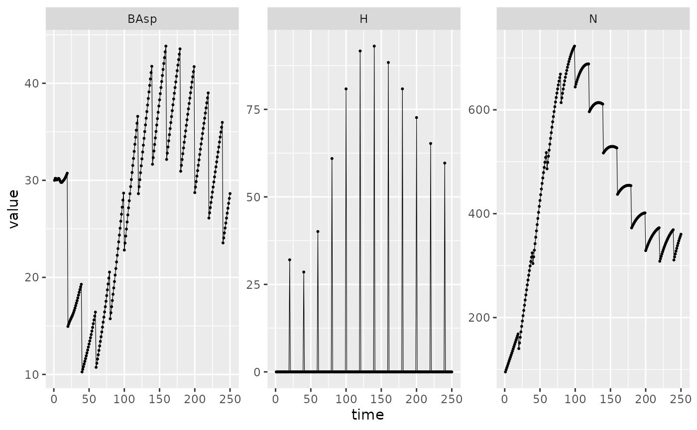
Uneven scenario
Theory
Uneven-aged harvest scenario consist in harvesting trees in all size classes with the objective to reach a stable size structure with continuous replacing of large mature trees. This scenario depends on the basal area of the stand and the size distribution of the tree. This should lead to stands with uneven size distribution.
Monospecific case
Harvest proportion
We note \(P_{cut}\) the global harvest proportion which will determine the amount of basal area to be harvested.
\[ P_{cut} = \left\lbrace \begin{array}{ll} 0 & if (BA_{stand} - BA_{target}) < \Delta BA_{min}\\ min(\frac{BA_{stand}-BA_{target}}{BA_{stand}}, P_{max}) & if (BA_{stand} - BA_{target}) \geq \Delta BA_{min} \end{array} \right\rbrace \]
For example, some numerical values of the parameters can be \(\Delta BA_{min} = 3 m^2ha^{-1}\), \(BA_{target} = 20, 25\) or \(30 m^2ha^{-1}\) (depending on species) and \(P_{max} = 0.25\).
Note that stand basal area \(BA_{stand}\) is computed only considering trees with a dbh above \(d_{th}\) (see below).
Harvest curve
Each tree harvest probability only depends on its diameter (\(d\)). There is a minimum diameter for harvest (\(d_{th}\)), harvest probability then increases with diameter until \(d_{ha}\) after which harvest probability is constant.
We therefore considered the harvesting function (which associates a \(dbh\) to an harvesting probability, building on the approach used in previous model such as Guillemot et al. (2014)).
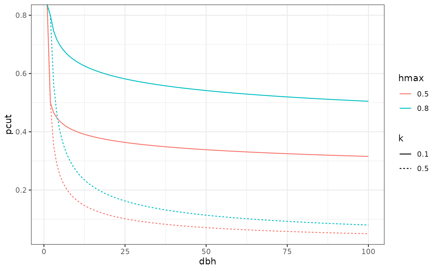
\[ h(d) = \left\lbrace \begin{array}{ll} 0 & \text{if } d < d_{th} \\ h_{max} (\frac{d - d_{th}}{d_{ha} - d_{th}})^{k} & \text{if } d_{th}\leq d < d_{ha} \\ h_{max} & \text{if } d \geq d_{ha} \end{array} \right\rbrace \]
The maximum harvesting for large tree \(h_{max}\) can be tuned so that the probability for a large tree to be harvested approaches 1 (for instance \(p = 0.999\)) after several harvesting operations: \(h_{max} = 1 - \sqrt[n]{1-p}\) with \(n\) the number of harvesting operations. Parameter \(k\) defines how quickly the harvesting rate increase from \(d_{th}\) to \(d_{ha}\).
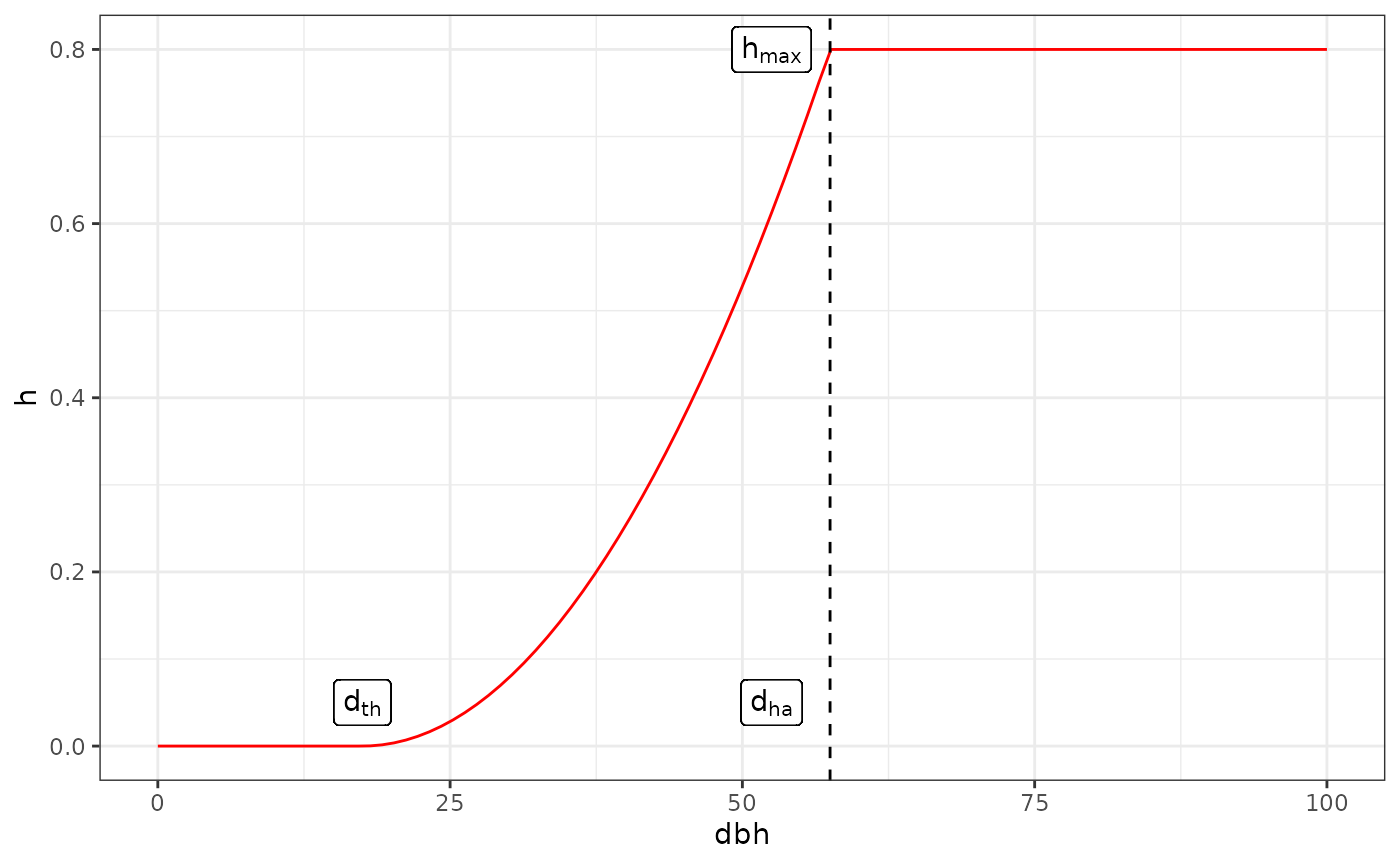
Harvest curve example, \(d_{th} = 17.5cm\), \(d_{ha}=57.5cm\), \(h_{max}=0.8\), \(k=2\).
Harvesting algorithm
The algorithm only target tree contributing to \(BA_{stand}\), that is the trees above \(d_{th}\). The algorithm start to harvest from largest trees to the smallest. The basal area harvested is function of \(P_{cut}\) and the density of trees in function of diameter \(\phi(x)\).
The basal area harvested is given by
\[ BA_{harv} = BA_{th} + BA_{ha} \] with \(BA_{ha}\) the basal area harvested for trees greater than \(d_{ha}\), and \(BA_{th}\) the basal area harvested for trees between \(d_{th}\) and \(d_{ha}\). The algorithm start to harvest from largest trees to the smallest.
The maximum of \(BA_{ha}\) is \(BA_{ha}^{max}\), and is given by:
\[ BA_{ha} = h_{max} \pi/4\int_{d_{ha}}^{d_{max}}x^2 \phi(x)dx \] where \(\phi\) is the density of trees.
\(\bullet\) If \(BA_{ha}^{max} >= P_{cut} \times BA_{stand}\), there is enough large trees (diameter above \(d_{ha}\)) so that the harvest will only concern large trees and \(BA_{th} = 0\). Here again the trees are harvested from the largest to the smallest.
We then find \(d_t\) (with \(d_{ha} < d_t < d_{max}\)) such that: \[ BA_{ha} = h_{max} \pi/4 \int_{d_{t}}^{d_{max}}x^2 \phi(x)dx = P_{cut} \times BA_{stand}\] Thus, the matreex package will cut the larger trees until \(P_{cut} \times BA_{ha} - targetBA <= 0\).
\(\bullet\) If \(BA_{ha}^{max} < P_{cut} \times BA_{stand}\), we first harvest \(BA_{ha}^{max}\) and then compute \(k\) such as: \(BA_{th} = P_{cut} \times BA_{stand} - BA_{ha}\).
With
\[ BA_{th} = \pi/4 \int_{d_{th}}^{d_{ha}}h(x)x^2 \phi(x)dx \]
Multispecific case
Abundance-based preference
As in the monospecific case, we define the global harvest rate \(P_{cut} = \frac{BA_{harv}}{BA_{stand}}\).
Here, \(BA_{stand}\) is divided between \(S\) species: \(BA_{stand} = \sum_{s=1}^{S} BA_{stand, s}\) and \(BA_{harv} = \sum_{s=1}^{S} BA_{harv, s}\)
We note the relative abundance of species \(s\), \(p_s =
\frac{BA_{stand, s}}{BA_{stand}}\), and the harvest rate of
species \(s\),
\(P_{cut, s} = \frac{BA_{harv, s}}{BA_{stand,
s}} = f(p_s) * P_{cut}\)
\(P_{cut, i} = \frac{BA_{stand, i} - BA_{harv, i}}{BA_{stand, i}} = f(p_i) * P_{cut}'\) By definition,
\[ \begin{array}{ll} BA_{harv} & = \sum_{s=1}^{S} BA_{harv, s} = \sum_{s=1}^{S} BA_{stand, s} * P_{cut, s} \\ & = BA_{stand} \sum_{s=1}^{S} p_s * f(p_s) *P_{cut} \\ & = BA_{stand} * P_{cut} \\ \end{array} \]
So that we have the constraint on \(f\): \(\sum_{s=1}^{S} p_s f(p_s) = 1\)
The case \(f(p_s) = 1\) works, which leads to \(P_{cut,s} = P_{cut}\). In that case the harvest rate is the same for every species \(s\).
More broadly, we can use the function \[f(p_s) = \frac{p_s^{\alpha - 1}}{\sum_{s=1}^{S} p_s ^{\alpha}}\], \(\forall \alpha > 0\)
For \(\alpha = 2\), we for example have
\[f(p_s) =\frac{p_s}{\sum_{s=1}^{S} p_s ^2} \] The shape of the function \(f\) depends on \(\alpha\). If \(\alpha = 1\), all species are harvested with the same rate irrespective of their relative abundance. For \(\alpha < 1\), the abundant species will be less harvested. Finally, for \(\alpha > 1\) the most abundant species will be harvested more, in a greater proportion than 1.
Favoured species
In some case, we may want to favour some species compared to others. We note \(q\) the set of \(Q\) species we want to favour, and \(p_q=\sum_{s=1}^{Q} p_s\) We first compute the harvest rate \(P_{cut,q}\) and \(P_{cut,1-q}\) for respectively the favoured/other species.
If \(p_q \geq 0.5\), we take \(P_{cut,q} = P_{cut,1-q} = P_{cut}\) (the species to be favoured are already dominant).
If \(p_q < 0.5\), we compute \(P_{cut,q}=f(p_q) P_{cut}\) and \(P_{cut,1-q}=f(1-p_q) P_{cut}\) with \(\alpha > 1\). By definition, we will get \(P_{cut,q} \leq P_{cut}\).
We then apply for each species \(s\) the harvest rate \(P_{cut,s} = P_{cut,q}\) or \(P_{cut,s}=P_{cut,1-q}\) depending on which group it belongs to.
Examples
All the parameters described above are input either in the
species(), forest() or
sim_deter_forest() functions. Additional parameter
dBAmin is the difference between BA and
targetBA under which an harvesting will not be
triggered.
When ploting the result, keep in mind the difference between
BAsp and BAstand. Only the second one will
match with targetBA, since during uneven harvesting, trees
below dth are excluded from computations.
Picea_Uneven <- species(IPM = Picea_ipm, init_pop = def_initBA(30),
                        harvest_fun = Uneven_harv,
                        harv_lim = c(dth = 175, dha = 575, hmax = 1))
Picea_for_Uneven <- forest(species = list(Picea = Picea_Uneven),
                      harv_rules = c(Pmax = 0.25, dBAmin = 3,
                                     freq = 5, alpha = 1))
set.seed(42) # The seed is here for initial population random functions.
Picea_sim_f20 <- sim_deter_forest(
    Picea_for_Uneven,
    tlim = 260, equil_time = 260, equil_dist = 10, equil_diff = 1,
    harvest = "Uneven", targetBA = 20, # We change the harvest and set targetBA.
    SurfEch = 0.03,
    verbose = TRUE
)
#> Starting while loop. Maximum t = 260
#> Simulation ended after time 260
#> BA stabilized at 22.70 with diff of 2.93 at time 260
#> Time difference of 1.37 secs
Picea_sim_f20  %>%
    dplyr::filter(var %in% c("BAsp", "BAstand", "N"), ! equil) %>%
    ggplot(aes(x = time, y = value)) +
    facet_wrap(~ var, scales = "free_y") +
geom_line(linewidth = .2) + geom_point(size = 0.4) 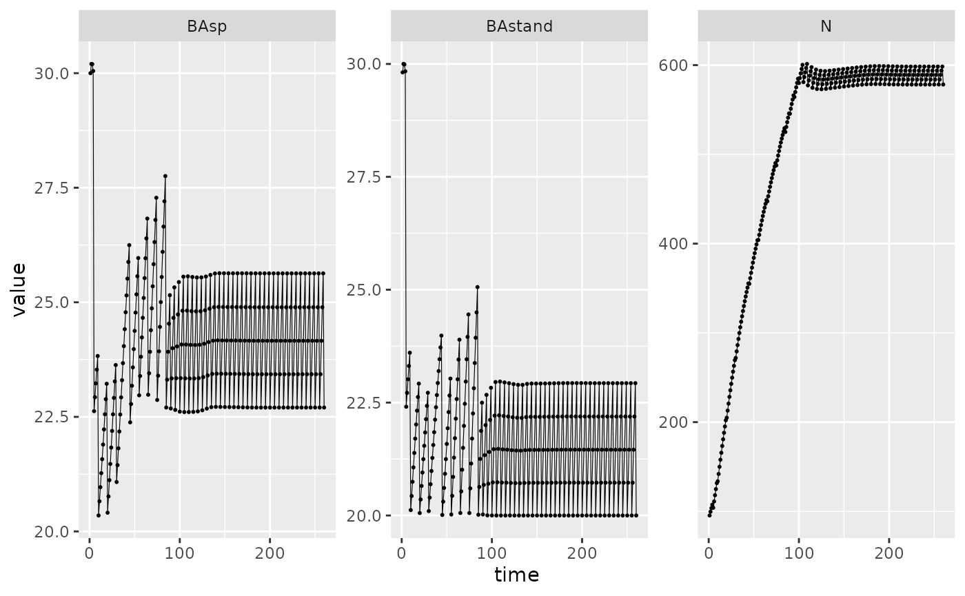
We notice that the basal area obtained by the simulation is higher than the targeted one. This can be explained by the fact that the cutting calculation is done on \(BA_{stand}\), which does not take into account individuals smaller than \(d_{th}\).
Even scenario
The objective of even harvesting is to apply harvesting typical of even-aged harvesting, where all trees started growing roughly at the same age, representing a single cohort. The tree are are harvested with thinning during the forest developpment till the final harvest. Thinning harvest are based on the distance to a self-thinning boundary. This self-thinning boundary is given for each species following :
\[N_{max} = e^{intercept+slope \cdot
log(Dg)}\] The species parameters are given in Aussenac et al. (2021) and inside the package with
rdi_coef table. \(Dg\) is
the mean quadratic diameter of trees.
data(rdi_coef)
rdi_coef <- drop(as.matrix(
    rdi_coef[rdi_coef$species == "Picea_abies",c("intercept", "slope")]
))
rdi_coef
#> intercept     slope
#>  12.51155  -1.65234
From this, we can compute the density index \(RDI = N / N_{max}\) with \(N\) the number of stems (Reineke (1933)).
The algorithm present in Even_harv is triggered if \(RDI > targetRDI\) and then harvest trees
depending on their diameters.
The degree of preference for small trees in the thinning harvest will depend on the parameter \(Kg\) (provided by the user), which is the ratio between the mean quadratic diameter of harvested trees \(Dg_d\) and the mean quadratic diameter \(Dg\) :
\[Kg = Dg^2_d / Dg^2\]
The algorithm present in Even_harv optimises two
parameters \(h_{max}\) and \(k\) of the harvesting function to reach
\(targetKg\) and \(targetRDI\).
\[h(d) = hmax * d^{-k}\]
Harvest curve example with various combination of hmax and k
The last parameter for an even harvested simulation is the final cut
time. The stand will be harvested with the previous rules at a given
frequency but at a certain point, the manager will harvest all trees and
plant new ones. This time is dependant on the species growth and
differents targets. The value is named final_harv in
sim_deter_forest() function.
Because the rdi coefficient depends on a species, it’s not possible to use multiple species forest with {matreex} package. Please contact authors if you need to use mutlispecific even harvesting.
Multispecific case
Because the species parameters are given in Aussenac et al. (2021) for a single species stand, computing \(N_{max}\) and \(Dg\) for multispecific stands is not straightforward.
The most simple approach to deal with is to sum the partial RDi of each species (which ignore interactive effect in the \(N_{max}\) between species) as done in Río et al. (2015) and Aussenac et al. (2021).
The stand RDI is the sum of the RDI of each species : \(RDI_{stand} = \sum_{s=1}^{S} N_s / N_{max,s}\)
The mean quadratic diameter is computed with all species at once :
\[Dg^2 = \frac{\sum_{s=1}^{S} \sum_{n=1}^{m} n_{s,n} \cdot dbh_{s,n}^2}{\sum_{s=1}^{S} N_{s}}\]
Examples
The rdi parameters are input in the species() function.
Calling forest() function is not different, only the
frequency of harvest will be used. The different targets
targetKg, targetRDI and
final_harv values are set when launching a simulation.
Picea_Even <- species(
    IPM = Picea_ipm, init_pop = def_init_even,
    harvest_fun = Even_harv, rdi_coef = rdi_coef,
    harv_lim = c(dth = 175, dha = 575, hmax = 1)
)

Picea_for_Even <- forest(species = list(Picea = Picea_Even),
                      harv_rules = c(freq = 10))
set.seed(42) # The seed is here for initial population random functions.
Picea_sim_f20 <- sim_deter_forest(
    Picea_for_Even,
    tlim = 100, equil_time = 100, equil_dist = 10, equil_diff = 1,
    harvest = "Even", targetRDI = 0.55, targetKg = 0.6,
    final_harv = 150, SurfEch = 0.03, verbose = TRUE
)
#> Starting while loop. Maximum t = 100
#> Simulation ended after time 100
#> BA stabilized at 42.66 with diff of 5.50 at time 100
#> Time difference of 0.859 secs
Picea_sim_f20  %>%
    dplyr::filter(var %in% c("BAsp", "N", "H"), ! equil) %>%
    ggplot(aes(x = time, y = value)) +
    facet_wrap(~ var, scales = "free_y") +
    geom_line(linewidth = .2) + geom_point(size = 0.4)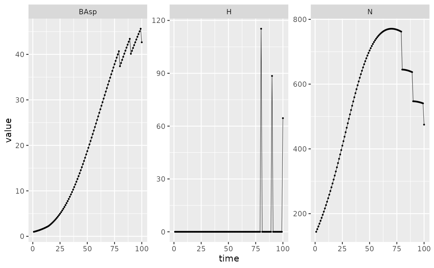
This chunk is used to add another species Abies alba and is no different than the creation of Picea abies species.
data("fit_Abies_alba")
Abies_ipm <- make_IPM(
    species = "Abies_alba",
    climate = climate, # this variable is defined at the top of the doc.
    fit = fit_Abies_alba,
    clim_lab = "optimum clim",
    mesh = c(m = 700, L = 90, U = get_maxdbh(fit_Abies_alba) * 1.1),
    BA = 0:80, # Default values are 0:200, smaller values speed up this vignette.
    verbose = TRUE
)
#> Launching integration loop
#> GL integration occur on 24 cells
#> midbin integration occur on 25 cells
#> Loop done.
#> Time difference of 38.1 secs

data(rdi_coef)
rdi_Ab <- drop(as.matrix(
    rdi_coef[rdi_coef$species == "Abies_alba",c("intercept", "slope")]
))

Abies_sp <- species(
    IPM = Abies_ipm, init_pop = def_init_even,
    harvest_fun = Even_harv, rdi_coef = rdi_Ab,
    harv_lim = c(dth = 175, dha = 575, hmax = 1)
)
PiAb_for_Even <- forest(
    species = list(Picea = Picea_Even, Abies = Abies_sp),
    harv_rules = c(freq = 10))
set.seed(42) # The seed is here for initial population random functions.
PiAb_sim_f20 <- sim_deter_forest(
    PiAb_for_Even,
    tlim = 200, equil_time = 200, equil_dist = 10, equil_diff = 1,
    harvest = "Even", targetRDI = 0.9, targetKg = 0.9,
    final_harv = 150, SurfEch = 0.03,
    verbose = TRUE
)
#> Starting while loop. Maximum t = 200
#> Simulation ended after time 200
#> BA stabilized at 28.00 with diff of 8.73 at time 200
#> Time difference of 1.98 secs
An additional function of the package is available for computing \(Kg\) and \(RDI\) after the simulations along time.
rdi_kg <- sim_rdikg(sim = PiAb_sim_f20, rdi_c = NULL)

PiAb_sim_f20 %>%
    filter(var %in% c("N", "BAsp", "H")) %>%
    select(species, time, var, value) %>%
    bind_rows(rdi_kg) %>%
    filter(var != "Dgcut2") %>%
    ggplot(aes(x = time, y = value, color = species)) +
    geom_line() +
    facet_wrap(~ var, scales = "free_y") +
    geom_hline(data = data.frame(yint=0.9,var=c("Kg", "rdi")),
               aes(yintercept = yint), linetype = "dashed")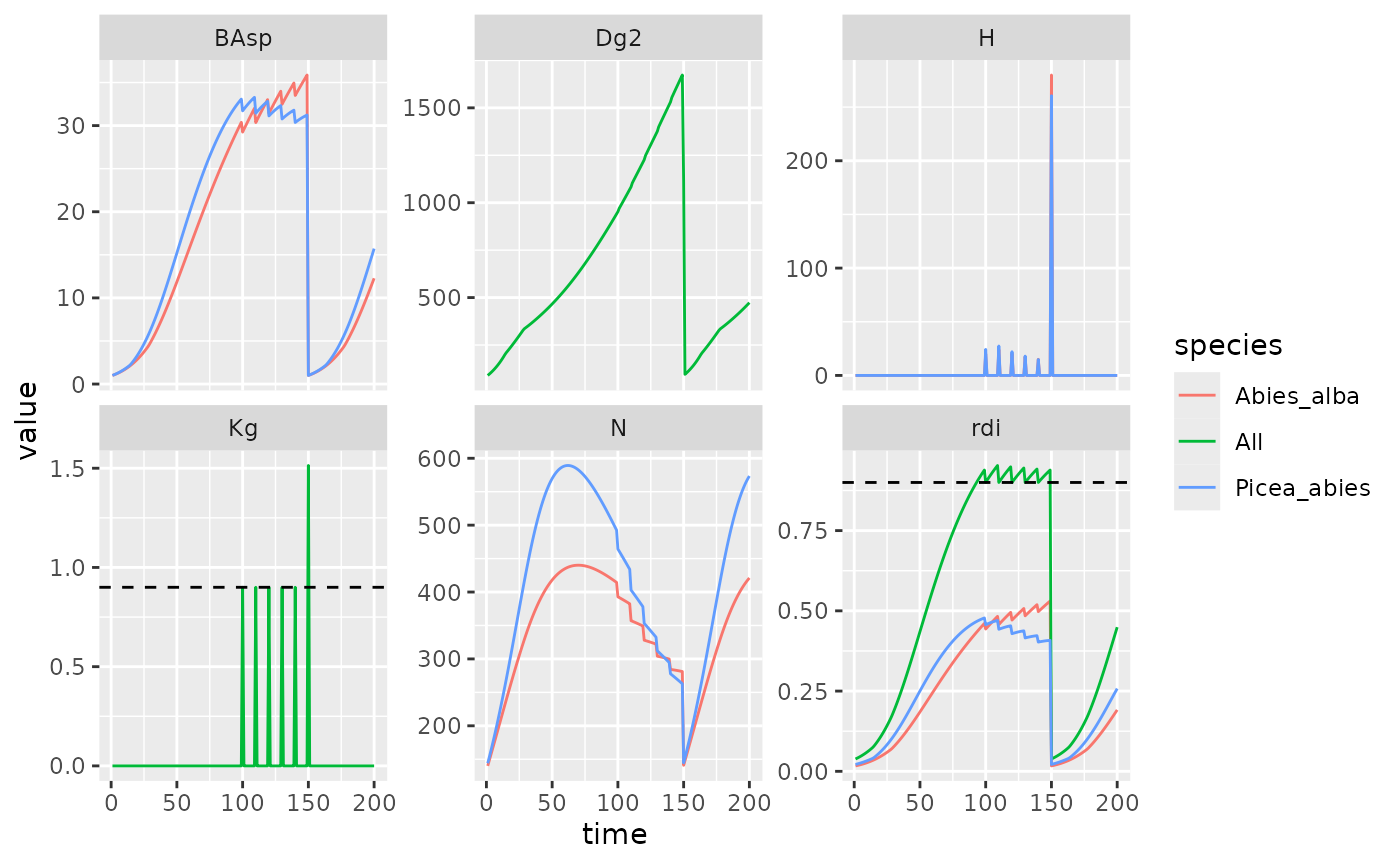
Summary variables for mutlispecific simulation with even harvesting function. Harvest frequence of 10 years and a final harvest at 150y. Dashed lines represent RDI and Kg targets. Both values where set to 0.9.